4 CATA Data — Analysis of Checked Terms
4.1 Introduction
This analysis is designed for CATA (Check-All-That-Apply) data, that is, when subjects check, from a predefined list, all the terms they consider appropriate to describe a stimulus. It answers two complementary questions: which terms characterise each stimulus and how the stimuli are globally organised according to their CATA profiles. The function produces a contingency table, a description of the stimuli according to the CATA terms, as well as a correspondence analysis followed by a classification of the stimuli, automatic by default.
Why not use a standard alternative?
CATA data are originally binary responses by subject and by term. A classical comparison of means is therefore not the most suitable tool for representing the global structure of these data. The function first aggregates the responses into a stimuli × terms contingency table, then applies methods suited to this structure: frequency description, correspondence analysis, and, when possible, classification.
4.2 Understanding what happens under the hood
4.2.1 Construction of the contingency table
The first step consists of grouping the responses by stimulus. The function sums the columns placed in the CATA field for each level of Stimulus Effect. This produces a table where rows are stimuli, columns are CATA terms, and each cell indicates how many times a term was checked for a given stimulus. This table is the basis for all subsequent outputs.
Note: this table can be copied into a spreadsheet file.
4.2.2 Description of stimuli by terms
From this contingency table, the function applies a frequency description procedure based on the threshold value defined in Significance threshold (%). For each stimulus, it identifies the terms that are significantly more or less frequent than in the whole table. This logic is close to a statistical description of profiles, but adapted here to checking frequencies rather than to continuous ratings. The same threshold is then applied to the description of clusters.
A term absent from the description table is not significantly associated with a stimulus at the chosen threshold. This may mean that it is checked fairly evenly across stimuli.
4.2.3 Correspondence analysis
If at least three variables are placed in the CATA field, the function performs a correspondence analysis on the contingency table. This method simultaneously represents the stimuli and the terms in the same factor space. Two stimuli that are close on the map tend to share similar CATA profiles; two terms that are close tend to be checked for similar stimuli. The axes summarise the main profile oppositions between stimuli and terms.
4.2.4 Classification of stimuli
Once the correspondence analysis has been computed, the function runs a hierarchical clustering on principal components (HCPC). By default, Number of clusters = -1 lets FactoMineR determine the number of groups automatically, but the user can also impose a number of clusters. The clustering uses the first CA dimensions defined by Number of dimensions for clustering; this setting is distinct from the factor plane displayed with X-axis and Y-axis. The percentages displayed on the HCPC map are expressed relative to the inertia of this retained clustering space and may therefore differ from those on the full CA map.
The function then produces a map of the stimuli according to their clusters and a description of the clusters using the same significance threshold as for the description of stimuli.
4.2.5 Minimum conditions for running the analysis
SEDA requires at least three CATA variables. With fewer than three attributes, the analysis stops. To construct a two-dimensional correspondence-analysis map, the aggregated table must also contain at least three stimuli and three informative CATA attributes.
CATA variables must be complete 0/1 indicators: 0 means that the term was not checked and 1 that it was checked. Missing values are not interpreted as unchecked responses and must be resolved before the analysis.
4.3 Expected data structure
The data must contain:
- one categorical column identifying the stimuli;
- at least three CATA columns coded as 0/1.
Each row corresponds to the evaluation of one stimulus by one subject. If 40 subjects evaluate 6 stimuli, the file generally contains one row per subject and per stimulus, with one column per CATA term.
Before running the analysis in jamovi, check in the Data tab that:
- the variable intended for Stimulus Effect is categorical;
- the variables intended for CATA are numeric and contain only
0and1; - no CATA response is missing: a missing value is not treated as
0; - at least three CATA terms are selected;
- at least three stimuli are actually observed to obtain the two-dimensional factor map.
4.4 Interface guide
The analysis appears in the menu SEDA > Fixed List of Attributes > Analysis of CATA Data. The interface includes two variable drop zones, an Instructions and R Code section, the Significance threshold (%) field, and two collapsible menus: Graphic Options and Clustering.
4.4.1 Variables to complete
4.4.1.1 Stimulus Effect
Role: identifies the stimuli to compare. Impact on the computation: this variable defines the rows of the contingency table and organises all descriptive and graphical outputs. Practical tip: use clear labels, because they will appear in the tables and graphs.
4.4.1.2 CATA
Role: groups together the terms from the CATA list. Impact on the computation: these variables define the columns of the contingency table; they are then used for stimulus description, correspondence analysis, and clustering. Practical tip: select at least three complete CATA variables coded as 0/1.
4.4.2 Instructions and R Code
4.4.2.1 Read me before running
Role: displays integrated help in the results. Impact on the computation: none. Practical tip: leave it checked during the first uses. It is enabled by default.
4.4.2.2 R code
Role: displays the R script corresponding to the analysis in an R Code output. Impact on the computation: none. Practical tip: enable this option to reproduce the analysis in the Rj Editor or continue working in R. It is disabled by default.
4.4.3 Significance threshold (%)
Role: defines the p-value threshold used to select terms characterising stimuli and clusters. Impact on the computation: this threshold affects the descfreq description tables but does not change the construction of the correspondence analysis or the clustering. Practical tip: the default value is 5%.
4.4.4 Graphic Options
4.4.4.1 X-axis and Y-axis
Role: choose the two correspondence-analysis dimensions displayed on the maps. Impact on the computation: they change the displayed plane, not the CA structure itself. Practical tip: start with X-axis = 1 and Y-axis = 2, the default values.
4.4.5 Clustering
4.4.5.1 Number of dimensions for clustering
Role: sets the number of first CA dimensions used by HCPC. Impact on the computation: clustering may therefore use more information than the displayed plane alone. The default value is 5; if fewer than five dimensions are available, SEDA uses all available dimensions. Practical tip: the axes chosen for the graph must be included among the dimensions used for clustering.
4.4.5.2 Number of clusters
Role: sets the number of stimulus groups. Impact on the computation: with the default value -1, FactoMineR determines the number of clusters automatically; an integer value of at least 2 imposes that number of groups. The requested number must remain lower than the number of stimuli. Practical tip: start with -1, and impose a number of groups only when there is an analytical reason to do so.
4.5 Step-by-step procedure
- Open your dataset in jamovi.
- In the Data tab, check that the stimulus variable is categorical and that the CATA variables are complete and coded 0/1.
- Open SEDA > Fixed List of Attributes > Analysis of CATA Data.
- Place the stimulus variable in Stimulus Effect.
- Place at least three terms in CATA.
- Leave Significance threshold (%) at 5% for a first trial.
- Keep X-axis = 1 and Y-axis = 2.
- Leave Number of dimensions for clustering = 5 and Number of clusters = -1 for an initial analysis.
- Start by reading Description of the Stimuli According to CATA.
- Then consult Representation of the Stimuli and the CATA, interpreting stimuli and terms relative to the axes.
- Read Representation of the Stimuli According to Clusters and then Description of the Clusters.
- Finally check Aggregated CATA Table — Stimuli × CATA Frequency Table, which contains the frequencies actually used in the computations.
- If necessary, change the factor plane or clustering settings, then check that your conclusions remain coherent.
4.6 Interpretation of results
4.6.1 Contingency table
This first table crosses stimuli in rows and CATA terms in columns. Each cell indicates the number of times a term was checked for a given stimulus.
| Element | Meaning |
|---|---|
| High value in a cell | The term was often checked for this stimulus |
| Row with several high values | The stimulus is associated with several frequent terms |
| Column high for almost all stimuli | Frequent term, but not necessarily discriminating |
Point of vigilance: a very frequent term is not automatically a characteristic term. If it is checked for almost all stimuli, it will contribute little to distinguishing them.
4.6.2 Description of the Stimuli According to CATA
This table describes each stimulus through the terms that are significantly associated with it, grouped by stimulus. Terms are sorted by decreasing V-test within each group.
| Element | Meaning |
|---|---|
| (first column) | Stimulus concerned |
| CATA | Characteristic term |
| Intern % | Percentage of use of the term for this stimulus |
| Global % | Overall percentage of use of the term |
| Intern frequency | Absolute frequency of the term for this stimulus |
| Global frequency | Total absolute frequency of the term |
| p | P-value of the test |
| V-test | Standardised intensity of the association |
- A positive V-test indicates that the term is checked more frequently for this stimulus than overall.
- A negative V-test indicates that it is checked less frequently — and is just as informative.
- A low p-value indicates a clearer characterisation.
A stimulus absent from this table does not have “no profile”; it is simply close to the mean profile of all stimuli at the chosen threshold.
4.6.3 Representation of the Stimuli and the CATA (available with at least 3 terms)
This graph is produced only if at least three terms are placed in CATA. It simultaneously represents the stimuli and the terms in the factor space derived from the correspondence analysis.
- Two close stimuli have similar CATA profiles.
- Stimuli and terms should be interpreted relative to the factor dimensions and the oppositions they structure; a direct distance between a stimulus and a term should not be read as an ordinary Euclidean distance.
- The percentage displayed on each axis indicates the share of total information captured by that dimension.
This map gives an overview, but it does not replace the descriptive table. The two should be read together.
4.6.4 Representation of the Stimuli According to Clusters (available with at least 3 terms)
This graph represents the stimuli according to the HCPC partition. With Number of clusters = -1, the partition is selected automatically; if a number of clusters is imposed, the map reflects that partition. Clustering uses the first dimensions defined by Number of dimensions for clustering, while X-axis and Y-axis determine the displayed plane. The percentages on the HCPC map refer to the retained clustering space, not to the full CA inertia.
- Stimuli in the same cluster have similar CATA profiles.
- Distant clusters correspond to more contrasted families of stimuli.
- This output helps summarise the global structure of the stimuli.
4.6.5 Description of the Clusters (available with at least 3 terms)
When the classification is available, the function also produces a table describing each cluster through the terms that are significantly associated with it, using the same logic as for the description of stimuli.
| Element | Meaning |
|---|---|
| (first column) | Group of stimuli concerned |
| CATA | Characteristic term |
| Intern % | Percentage of the term within the cluster |
| Global % | Overall percentage of the term |
| Intern frequency | Absolute frequency of the term within the cluster |
| Global frequency | Total absolute frequency of the term |
| p | P-value |
| V-test | Standardised intensity of the association |
This table is particularly useful for summarising the main families of stimuli, beyond the stimulus-by-stimulus details.
4.7 Example: the Giacalone_et_al_cata dataset
The Giacalone_et_al_cata dataset describes 9 beers evaluated by 74 consumers on 15 CATA items: here, the aim is to associate beers with particular occasions. It is used to illustrate the function outputs. The numerical values and graphics discussed below come directly from the analysis results. To load this dataset, open jamovi, click the icon in the top left corner, the three stacked lines, then Open → Data Library → SEDA.
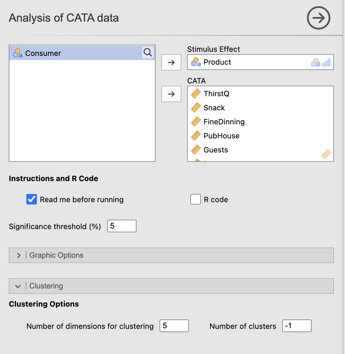
4.7.1 Example settings
To reproduce this example, use the following values.
| Option | Value |
|---|---|
| Stimulus Effect | Product |
| CATA | all CATA items from ThirstQ to Concert |
| Significance threshold (%) | 5 |
| X-axis / Y-axis | 1 / 2 |
| Number of dimensions for clustering | 5 |
| Number of clusters | -1 (automatic) |
Figure 4.1 shows the configuration used for the CATA example.
4.7.2 Analysis of the Description of the Stimuli According to CATA table
The table allows a stimulus-by-stimulus reading with test values and actual frequencies.
GMA is significantly characterised by Rugby (V-test = 3.95, p < .001; 11.61% versus 7.08% overall) and CampingFishing (2.73, p = 0.006). Conversely, it is under-represented by Gift (V-test = -4.36), Treat (-3.84), and FineDinning (-3.51) — all highly significant.
LR has the profile most strongly marked by Rugby in the whole set (V-test = 5.74, p < .001; 15.24% versus 7.08% overall) and CampingFishing (2.83). It is under-represented by Guests (-4.77), FineDinning (-3.91), Treat (-3.74), and Gift (-3.50).
SSA stands out from all other stimuli by the intensity of its positive associations: Gift (V-test = 6.43, p < .001; 13.41% versus 4.21% overall), FineDinning (6.09), Treat (4.53), Achievement (3.71), and Guests (2.72). Conversely, it is strongly under-represented by Rugby (-4.29), ThirstQ (-3.63), Work (-3.01), CampingFishing (-2.88), and TV (-2.80). It is the stimulus whose profile differs most clearly from the mean.
SC is more strongly linked to Rugby (2.82) and ThirstQ (2.69), and is under-represented by PubHouse (-2.67), Treat (-2.58), and Gift (-2.55).
HPW is more strongly associated with Treat (V-test = 2.41) and Gift (2.21), and is under-represented by Rugby (-3.29). PKB is more strongly associated with Gift (2.60) and Treat (2.10); no negative term reaches the 5% threshold for this stimulus.
MBB mainly stands out through PubHouse (2.62) and is negatively distinguished by ThirstQ (-2.35) and Rugby (-2.19).
STG is characterised only by Rugby on the negative side (-2.75, p = 0.006).
4.7.3 Analysis of the Representation of the Stimuli and the CATA graph
Figure 4.2 shows the factorial representation used in this example.
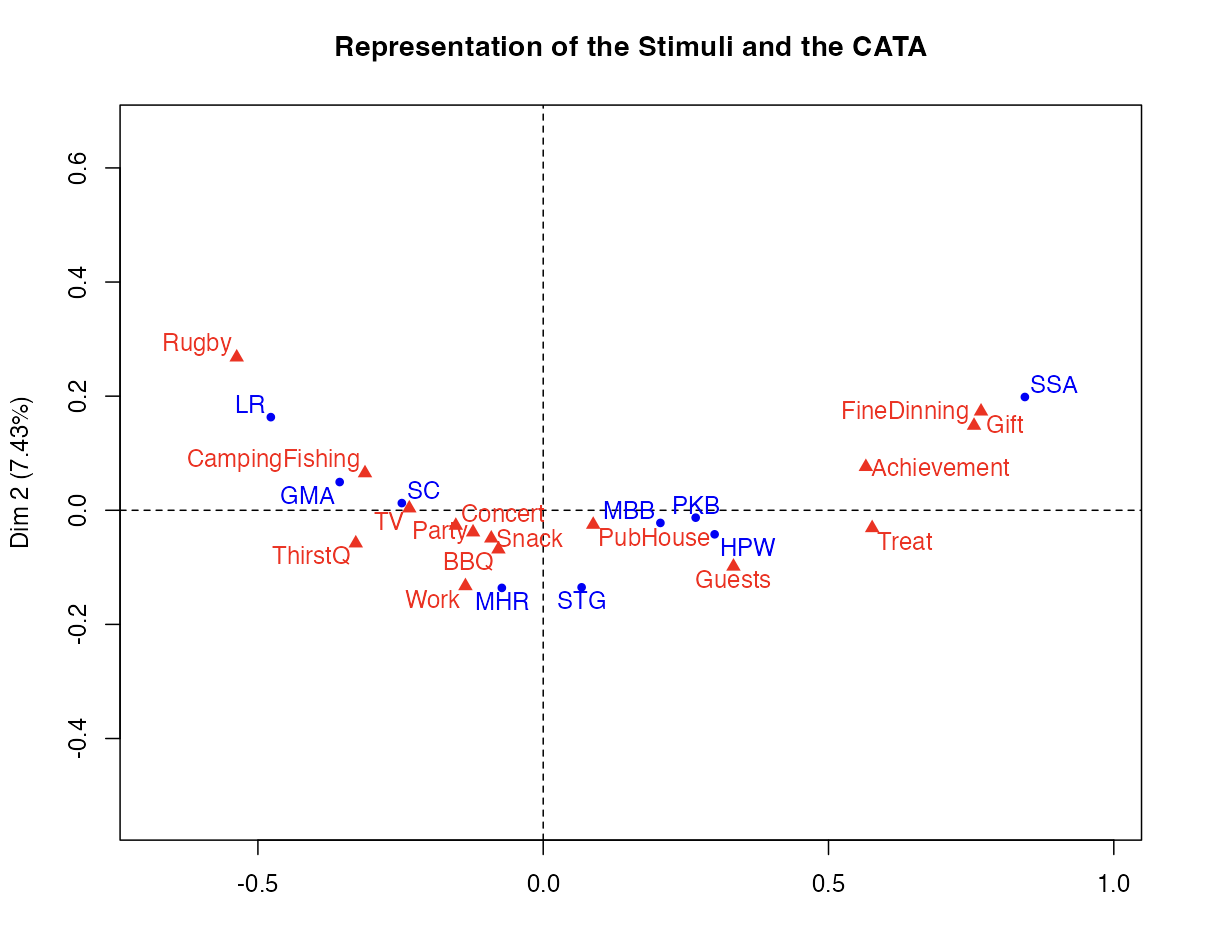
The first dimension explains 85.59% of the inertia — a remarkably high value, meaning that the main opposition between stimuli is very strong and very readable on the horizontal axis. The second dimension explains only 7.43%, but refines secondary distinctions.
On the map, SSA is located very clearly on the right, isolated near Gift, FineDinning, and Achievement. On the left are grouped LR, GMA, and SC, close to Rugby and CampingFishing. MBB, HPW, PKB, MHR, and STG occupy a central or slightly right-hand position, between the two poles. On the second dimension, LR is located slightly higher than GMA and SC, which reflects its stronger association with Rugby.
4.7.4 Analysis of the Representation of the Stimuli According to Clusters and the Description of the Clusters graph and table
Figure 4.3 shows the partition of the stimuli retained by the classification.
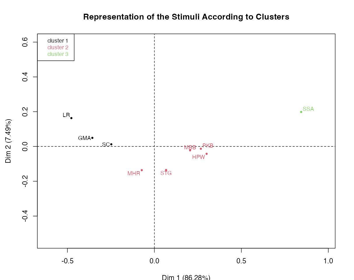
The automatic classification retains three clusters:
Cluster 1 (black): LR, GMA, and SC — positively characterised by Rugby (V-test = 9.12, p < .001), CampingFishing (4.86), ThirstQ (3.81), and TV (3.01), and under-represented notably by Gift (-6.97), Treat (-6.81), FineDinning (-6.21), and Guests (-4.67). This cluster corresponds to the pole most strongly associated with sports and outdoor contexts.
Cluster 2 (red): MBB, HPW, PKB, MHR, and STG — positively characterised by Treat (V-test = 3.52), Guests (2.86), Gift (2.18), PubHouse (2.15), and Achievement (2.05), and under-represented by Rugby (-7.07), CampingFishing (-3.34), and ThirstQ (-2.02). This cluster groups beverages more associated with social or treat-related contexts and less with sports and outdoor contexts.
Cluster 3 (green): SSA alone — positively characterised by Gift (V-test = 6.43), FineDinning (6.09), Treat (4.53), Achievement (3.71), and Guests (2.72), and negatively by Rugby (-4.29), ThirstQ (-3.63), Work (-3.01), CampingFishing (-2.88), TV (-2.80), and Party (-2.39). The profile of SSA is singular enough to form a cluster on its own.
4.7.5 Synthetic interpretation
This example clearly shows the value of the function. It does not merely show that an item is often checked: it shows for which stimuli it is truly characteristic, how the stimuli are globally opposed, and which main profiles emerge from the set of responses. Here, the major opposition — captured at 85.59% by the first dimension — contrasts beverages associated with sports and outdoor contexts (Rugby, CampingFishing) with beverages perceived as more sophisticated (Gift, FineDinning, Treat). SSA is a special case, with a profile singular enough to form a cluster on its own.
What we take away from this example: CATA analysis makes it possible to move from simple checking frequencies to a structured reading of the oppositions between stimuli and the main profiles that emerge from them.
4.8 From jamovi to the Rj Editor
Once the Rj Editor has been configured to use System R as described in Chapter 1, check R code to display the script corresponding to the analysis. The dataset currently open in jamovi is available as data.
For CATA, the script loads FactoMineR, aggregates the 0/1 indicators by stimulus, then uses descfreq() for characterisation, CA() for correspondence analysis, and HCPC() for clustering. The X-axis / Y-axis, Number of dimensions for clustering, and Number of clusters settings are carried into the generated code.
The script also uses graphics options suited to the Rj Editor so that no external graphics device is opened. No additional setting is required.
4.9 Practical tips
- Start with Significance threshold (%) = 5%; increase to 10% if the description tables are too empty.
- Always check the contingency table before interpreting the graphs.
- At least three CATA terms and three observed stimuli are required to construct the two-dimensional factor map.
- A negative V-test is just as informative as a positive V-test: it indicates that a term is checked significantly less often for a stimulus than for the others.
- Do not overinterpret the absence of a stimulus from the descriptive table: it may simply have a profile close to the mean profile.
- Classification is automatic by default (
Number of clusters = -1), but you can impose a number of groups; always assess its relevance by cross-reading the map and the cluster description. - Read the correspondence map together with the description table: the map gives an overview, while the table provides the details.
- CATA columns must contain only
0and1and must not contain missing values; a missing value is not treated as an unchecked response.
4.10 In summary
This analysis transforms CATA responses into a structured reading of the CATA profiles of stimuli. It combines a contingency table, a statistical description of stimuli, a correspondence analysis, and a classification, automatic by default. Its main value is to move from a simple accumulation of checkmarks to a view of the stimuli that is simultaneously descriptive, factorial, and typological.