5 JAR Data — Defect and Penalty Analysis

5.1 Introduction

This analysis is designed for JAR (Just About Right) data, in which subjects evaluate a sensory attribute relative to an ideal level, for example too little / just about right / too much. It identifies deviations from the JAR level, estimates their frequency, and studies their relationship with liking.

SEDA provides two complementary penalty views. The first is a global view, based on SensoMineR::JAR, which estimates the importance of defects across the whole product space. The second is a classical product-specific analysis, which compares, for a given product, the liking of consumers who rate an attribute JAR with that of consumers who rate it below or above JAR.

Why not use a simple mean liking score?

A mean liking score by product does not show which sensory deviations are associated with a decrease in liking. Likewise, the frequency of JAR responses alone does not indicate whether a frequent defect is actually penalising. The value of the analysis is therefore to combine three different pieces of information: defect frequency, size of the liking loss, and statistical uncertainty around that loss.

5.2 Understanding what happens under the hood

5.2.1 Checking and grouping the JAR coding

The value entered in Coding of the JAR level must exactly match the category representing the ideal level in every selected JAR attribute. The default value is jar.

For the classical product-specific analysis, SEDA then groups the other categories into two directions:

Below JAR;
Above JAR.

This grouping uses the expressions defined in Below-JAR keywords and Above-JAR keywords. The first output to inspect is therefore JAR Coding Used for the Classical Penalty Analysis. A level shown as Unclassified should be resolved before interpreting the classical analysis; otherwise, the corresponding attribute is excluded from that part of the analysis.

5.2.2 Distribution of JAR responses

SEDA calculates, for each product and attribute, the percentages of consumers Below JAR, JAR, and Above JAR. This output describes how frequent the deviations are, but does not yet indicate whether they reduce liking.

5.2.3 Global multidimensional penalties

SensoMineR::JAR estimates penalties using all products simultaneously. In SEDA, they are presented as Mean drop values: a positive value means that the defect is associated with a loss of liking across the global product space.

These coefficients are global and are not product-specific estimates. SEDA then combines them with the frequency of each defect in each product in Global Defects Applied to Each Product.

A row receives Priority = Yes when three conditions are met:

the percentage of consumers reaches Consumer threshold (%);
the Global mean drop reaches Mean-drop threshold;
the global penalty p-value is below 0.05.

The two interface thresholds are therefore practical decision aids, not substitutes for the p-value.

5.2.4 Classical product-specific penalty analysis

SEDA also calculates, separately for each product, attribute, and direction (Below JAR or Above JAR):

Mean drop = Mean liking JAR − Mean liking non-JAR

A positive value therefore means that consumers perceiving the deviation give a lower mean liking score than consumers rating the attribute JAR.

For each comparison, SEDA reports:

the percentage of consumers concerned;
mean liking in the JAR group;
mean liking in the non-JAR group;
Mean drop;
its 95% confidence interval;
the p-value.

This analysis is genuinely product-specific and complements the global penalty view.

5.2.5 Multivariate synthesis of defects

Finally, SEDA constructs a products × non-JAR categories frequency table, describes it with descfreq(), and performs a correspondence analysis.

The product description deliberately uses a permissive exploratory threshold (proba = 0.5). It is intended to reveal the categories structuring the space and should not be interpreted as a conventional 5% significance filter.

The correspondence map summarises the product × defect structure. As in the CATA chapter, products and defects should be interpreted relative to the factor dimensions; a direct row-to-column distance is not an ordinary Euclidean distance. Proximity on this map is not, by itself, evidence of a liking penalty.

5.3 Expected data structure

The data must contain:

one categorical column for Stimulus Effect;
one categorical column for Subject Effect;
one numeric column for Liking Variable;
one or more nominal columns for Sensory Attributes.

Each row corresponds to one subject evaluating one stimulus.

Before running the analysis, check that:

Stimulus Effect contains at least two observed products;
Subject Effect contains at least two observed subjects;
Liking Variable is numeric and contains enough finite observations;
JAR variables are defined as Nominal in jamovi;
every JAR attribute contains the category specified in Coding of the JAR level;
every JAR attribute has at least two observed response levels;
the variables used for Stimulus, Subject, Liking, and JAR attributes are distinct.

5.4 Interface guide

The analysis appears in SEDA > Fixed List of Attributes > Analysis of JAR Data. The interface includes four variable drop zones, an Instructions and R Code section, the Coding of the JAR level field, and a Classical Penalty Analysis section.

5.4.1 Variables to complete

5.4.1.1 Stimulus Effect

Role: identifies the products to analyse. Impact on the computation: this variable defines the products used in both global and product-specific analyses. Practical tip: use short, explicit labels.

5.4.1.2 Subject Effect

Role: identifies the subjects. Impact on the computation: this variable is used by the global JAR analysis and structures individual observations. Practical tip: ensure that each subject keeps the same identifier throughout the dataset.

5.4.1.3 Liking Variable

Role: contains the liking score used to calculate penalties. Impact on the computation: all liking losses are expressed in the units of this variable. Practical tip: use the same liking scale for all products.

5.4.1.4 Sensory Attributes

Role: groups the JAR variables. Impact on the computation: each variable is used in the global, product-specific, and multivariate analyses. Practical tip: variables must be nominal, even when their categories conceptually follow an order such as too little / JAR / too much.

5.4.2 Instructions and R Code

5.4.2.1 Read me before running

Role: displays integrated help. Impact on the computation: none. It is enabled by default.

5.4.2.2 R code

Role: displays the R script reproducing the analysis. Impact on the computation: none. Enable it to continue the analysis in the Rj Editor. It is disabled by default.

5.4.3 Coding of the JAR level

Role: gives the exact label of the JAR category. Impact on the computation: this category is used as the reference in all analyses. Practical tip: the default is jar; match the label in the data exactly.

5.4.4 Classical Penalty Analysis

5.4.4.1 Consumer threshold (%)

Role: defines the percentage of consumers above which a defect is considered frequent enough for an operational reading. Default: 20%. Important: this is a decision aid, not a significance threshold.

5.4.4.2 Mean-drop threshold

Role: defines the liking loss above which an effect is considered large enough for an operational reading. Default: 1. Important: this threshold concerns effect size, not statistical uncertainty.

5.4.4.3 Below-JAR keywords

Role: defines the words or expressions used to recognise categories below the JAR level. The default is too low|not enough|too weak|plain|low.

5.4.4.4 Above-JAR keywords

Role: defines the words or expressions used to recognise categories above the JAR level. The default is too high|too much|too strong|vivid|high.

Practical tip: always start by checking JAR Coding Used for the Classical Penalty Analysis. If a category is Unclassified, adapt the keywords before interpreting product-specific results.

5.5 Step-by-step procedure

Open the dataset in jamovi.
Check that Stimulus Effect and Subject Effect are categorical, Liking Variable is numeric, and JAR attributes are nominal.
Open SEDA > Fixed List of Attributes > Analysis of JAR Data.
Fill Stimulus Effect, Subject Effect, Liking Variable, and Sensory Attributes.
Check Coding of the JAR level.
Leave Consumer threshold (%) = 20 and Mean-drop threshold = 1 for a first reading.
Check Below-JAR keywords and Above-JAR keywords.
Read JAR Coding Used for the Classical Penalty Analysis and resolve any Unclassified category.
Read Distribution of JAR Responses by Product and Attribute.
Examine Global Multidimensional Penalties (All Products) and then Global Defects Applied to Each Product.
Use Global Penalty Context for Each Product to see which products are exposed to globally important defects.
Then read Product-Specific Classical Penalty Analysis and the Product-Specific Penalty Plots.
Finish with Description of the Products According to Defects, Representation of the Products and the Defects, and Frequency Table Used for the Correspondence Analysis.
Cross-read frequency, mean-drop magnitude, and statistical uncertainty before retaining a product-optimisation lever.

5.6 Interpretation of results

5.6.1 JAR Coding Used for the Classical Penalty Analysis

This table is the essential preliminary check. For each attribute and original response level, it shows whether SEDA uses it as Below JAR, JAR, Above JAR, or Unclassified.

An Unclassified category should not be ignored: the corresponding attribute is excluded from the classical product-specific analysis until its coding is resolved.

5.6.2 Distribution of JAR Responses by Product and Attribute

For each product and attribute, this table reports:

Below JAR (%);
JAR (%);
Above JAR (%);
N.

It answers the question: how many consumers actually perceive the deviation? It does not measure its impact on liking.

5.6.3 Global Multidimensional Penalties (All Products)

This table contains the coefficients from SensoMineR::JAR:

Column	Interpretation
Defect	Non-JAR category
Mean drop	Global liking loss associated with the defect
Std. Error	Estimation uncertainty
p	Associated statistical evidence

Mean drop is presented so that a positive value corresponds to a loss of liking.

Point of vigilance: these coefficients are estimated across all products. They should not be described as product-specific penalties.

5.6.4 Global Defects Applied to Each Product

This table combines the local frequency of a defect in each product with its Global mean drop.

Column	Interpretation
Consumers (%)	Defect frequency in the product
Global mean drop	Globally estimated mean drop
p	Global penalty p-value
Priority	`Yes` if frequency, mean drop, and p-value meet the criteria

With the default settings, Priority = Yes therefore means at least 20% of consumers concerned, a mean drop of at least 1, and p < .05.

5.6.5 Global Penalty Context for Each Product

These graphs provide the native SensoMineR visualisation of the global penalty in the context of each product. They help identify products exposed to globally important defects, but the y-coordinate does not thereby become a product-specific penalty.

5.6.6 Product-Specific Classical Penalty Analysis

This table answers a different question: for this specific product, do consumers perceiving the attribute as non-JAR like the product less than consumers rating it JAR?

Column	Interpretation
Product	Product concerned
Attribute	JAR attribute
Direction	Below JAR or Above JAR
Consumers (%)	Percentage of consumers in that direction
Mean liking JAR	Mean liking in the JAR group
Mean liking non-JAR	Mean liking in the relevant non-JAR group
Mean drop	Mean liking JAR − Mean liking non-JAR
CI 95% low / high	95% confidence interval for the mean drop
p	Test p-value

A positive Mean drop indicates a liking loss associated with the deviation for that product.

5.6.7 Product-Specific Penalty Plots

For each product:

the x-axis represents Consumers concerned (%);
the y-axis represents Mean drop in liking;
the vertical dashed line corresponds to the Consumer threshold;
the horizontal dashed line corresponds to the Mean-drop threshold;
symbols distinguish Below JAR from Above JAR;
* indicates p < .05;
vertical intervals show the 95% confidence interval.

A defect in the high-frequency / high-mean-drop region may be an operational lever, but confidence intervals and p-values should remain part of the decision.

5.6.8 Description of the Products According to Defects

This table describes the non-JAR categories structuring each product profile. It deliberately uses a very permissive exploratory threshold in this multivariate synthesis. A category displayed with p > .05 is therefore not “significant at 5%”; it is retained to help interpret the structure of the space.

5.6.9 Representation of the Products and the Defects

This map comes from correspondence analysis of the products × defects table. Two nearby products have similar defect profiles. For product-to-defect relationships, interpret directions and factor dimensions rather than a direct row-to-column distance.

This map describes the structure of defects; it is not a test of liking penalty.

5.6.10 Frequency Table Used for the Correspondence Analysis

This table contains the products × non-JAR-category frequencies used by descfreq() and correspondence analysis. It is a useful audit output for understanding exactly which aggregated data feed the multivariate synthesis.

5.7 Example: the milkshake dataset

The milkshake dataset contains three milkshakes, 284, 859, and 972, evaluated by 47 consumers using several JAR attributes related to color, fluidity, odors, sweetness, acidity, texture, and taste. To load the dataset, open jamovi, click the icon in the top left corner, then Open → Data Library → SEDA.

This example is especially useful because it shows that the global and product-specific views can lead to complementary diagnoses.

5.7.1 Example settings

Option	Value
Stimulus Effect	Product
Subject Effect	Panelist
Liking Variable	Liking
Sensory Attributes	all JAR variables from Color to Taste_Van
Coding of the JAR level	`jar`
Consumer threshold (%)	20
Mean-drop threshold	1
Below-JAR keywords	`too low\|not enough\|too weak\|plain\|low`
Above-JAR keywords	`too high\|too much\|too strong\|vivid\|high\|too_fluid`

Figure 5.1 shows the configuration used for the JAR example.

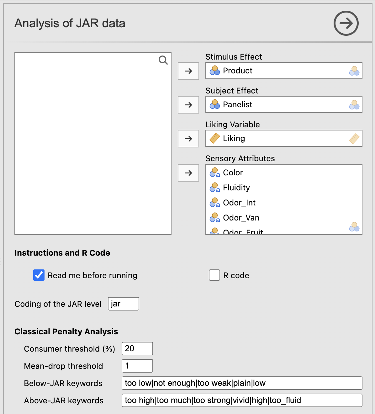
Figure 5.1: Configuration of the JAR analysis in jamovi for the *milkshake* dataset.

The final term added to Above-JAR keywords correctly classifies Too_fluid as Above JAR. SEDA accepts both Too_fluid and too fluid: original labels and their normalised forms are recognised.

5.7.2 Check the JAR coding first

The JAR Coding Used for the Classical Penalty Analysis table confirms that all response levels used in this example are classified as Below JAR, JAR, or Above JAR. For Fluidity, Not_enough_fluid is classified as Below JAR and Too_fluid as Above JAR.

This check matters because the classical product-specific analysis can only be interpreted when the non-JAR categories of the attribute are correctly grouped.

5.7.3 Distribution of JAR responses

The Distribution of JAR Responses by Product and Attribute table identifies the most frequent deviations.

For 284, Below JAR responses are particularly frequent for Odor_Van (59.57%), Texture (57.45%), and Odor_Int (53.19%), while 46.81% of consumers rate Fluidity Above JAR.

For 859, two deviations dominate: 80.85% of consumers are Below JAR for Texture and 70.21% are Above JAR for Fluidity.

For 972, 55.32% are Below JAR for Odor_Int, 42.55% are Above JAR for Sweetness, and 38.30% are Above JAR for Fluidity.

These percentages describe prevalence. They do not by themselves show that the deviations reduce liking.

5.7.4 Global multidimensional penalties

In Global Multidimensional Penalties (All Products), only one defect is significant at the 5% level: Too_much_odor_fruit, with Mean drop = 2.68 and p = 0.018.

Several other effects have notable mean drops without reaching the 5% threshold, for example Too_much_acidity (4.02, p = 0.082), Too_much_texture (1.78, p = 0.089), and Not_enough_acidity (1.03, p = 0.087).

In SEDA, a positive Mean drop represents a loss of liking.

5.7.5 Global Defects Applied to Each Product

With Consumer threshold = 20% and Mean-drop threshold = 1, no row receives Priority = Yes.

Too_much_odor_fruit is the only globally significant defect, but it concerns only 6.38% of consumers for 284, 4.26% for 859, and 4.26% for 972. It is therefore statistically associated with a liking loss across the global product space, but it is too rare within each product to exceed the practical 20% threshold.

Conversely, Too_fluid is very frequent — 46.81% for 284, 70.21% for 859, and 38.30% for 972 — but its Global mean drop = 0.45 with p = 0.275. High prevalence and global penalty therefore do not necessarily coincide.

5.7.6 Classical product-specific penalties

The Product-Specific Classical Penalty Analysis provides a directly local view.

For 284, several deviations are associated with a significant liking loss:

Odor_Fruit — Below JAR: 46.81% of consumers, Mean drop = 1.00, 95% CI [0.04, 1.96], p = 0.042;
Odor_Fruit — Above JAR: 6.38%, Mean drop = 2.27, 95% CI [0.47, 4.08], p = 0.016;
Sweetness — Below JAR: 21.28%, Mean drop = 1.22, 95% CI [0.04, 2.40], p = 0.044;
Texture — Below JAR: 57.45%, Mean drop = 1.06, 95% CI [0.10, 2.02], p = 0.032.

For Fluidity — Above JAR, 46.81% of consumers are concerned, but Mean drop is only 0.69 with p = 0.182. The deviation is therefore frequent without being clearly penalising for 284.

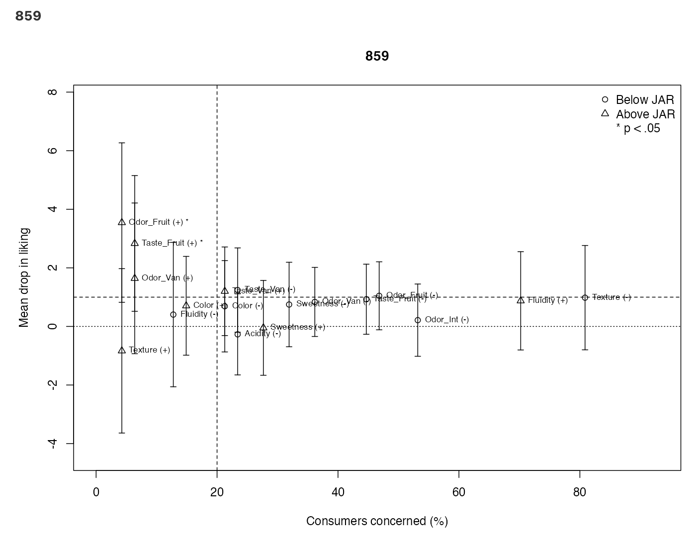
For 859, Fluidity — Above JAR gives a particularly instructive result: 70.21% of consumers are concerned, but Mean drop is only 0.87, p = 0.298. Likewise, Texture — Below JAR concerns 80.85% of consumers but has Mean drop = 0.98, p = 0.272. These two deviations are extremely frequent without a clearly established hedonic impact in the product-specific analysis.

The two significant effects for 859 instead concern very small groups:

Odor_Fruit — Above JAR: 4.26%, Mean drop = 3.55, p = 0.013;
Taste_Fruit — Above JAR: 6.38%, Mean drop = 2.83, p = 0.019.

The effects are large but rare, which limits their operational priority.

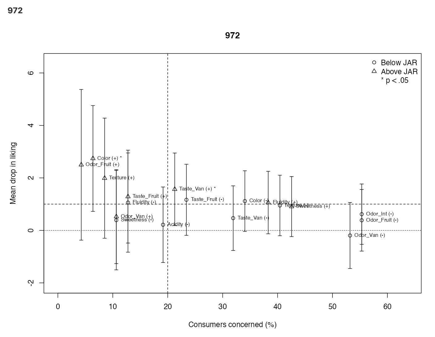
For 972, Fluidity — Above JAR concerns 38.30% of consumers with Mean drop = 1.06 and p = 0.080: the signal is compatible with a liking loss but remains insufficient to conclude at the 5% level.

Two other effects are significant:

Color — Above JAR: 6.38%, Mean drop = 2.74, p = 0.009;
Taste_Van — Above JAR: 21.28%, Mean drop = 1.57, 95% CI [0.19, 2.95], p = 0.028.

The second is especially useful because it combines frequency above 20%, mean drop above 1, and p < .05. Taste_Van — Above JAR is therefore the clearest product-specific optimisation lever for 972.

5.7.7 What the product-specific plots show

The Product-Specific Penalty Plots make this logic visible: the vertical line marks 20% of consumers and the horizontal line marks a mean drop of 1.

For 284, several significant points lie in or near the upper-right region, especially lack of texture, sweetness, and fruity odor.

For 859, Fluidity — Above JAR and Texture — Below JAR lie far to the right of the graph, meaning that they are very frequent, but remain below or around the mean-drop threshold and are not significant. The two significant effects instead have large mean drops but lie far to the left because they concern few consumers.

Figure 5.2 shows the product-specific penalty plot for product 859.

Figure 5.2: Product-specific penalty plot for product 859.

For 972, Taste_Van — Above JAR combines frequency, effect size, and statistical evidence, whereas Fluidity — Above JAR is a more uncertain signal.

Figure 5.3 shows the product-specific penalty plot for product 972.

Figure 5.3: Product-specific penalty plot for product 972.

These plots show why frequency, effect size, and uncertainty should be considered together.

5.7.8 Multivariate synthesis of defects

The Description of the Products According to Defects table uses the exploratory threshold proba = 0.5. The displayed rows should therefore not all be described as “significant at 5%”.

Product 859 is mainly oriented toward Texture = Not_enough_texture (V-test = 1.92, p = 0.055) and Fluidity = Too_fluid (1.75, p = 0.080), while Color = A_little_plain (-2.05, p = 0.040) and Odor_Van = Not_enough_odor_van (-1.97, p = 0.049) are under-represented.

Product 972 is notably oriented toward Sweetness = Too_much_sweetness (V-test = 1.71, p = 0.087), while Texture = Not_enough_texture is under-represented (V-test = -1.80, p = 0.072).

Product 284 shows a less marked structure; its strongest positive category is Color = A_little_plain (V-test = 1.32, p = 0.187).

5.7.9 Representation of the Products and the Defects

Figure 5.4 shows the factorial structure of the products and the defects.

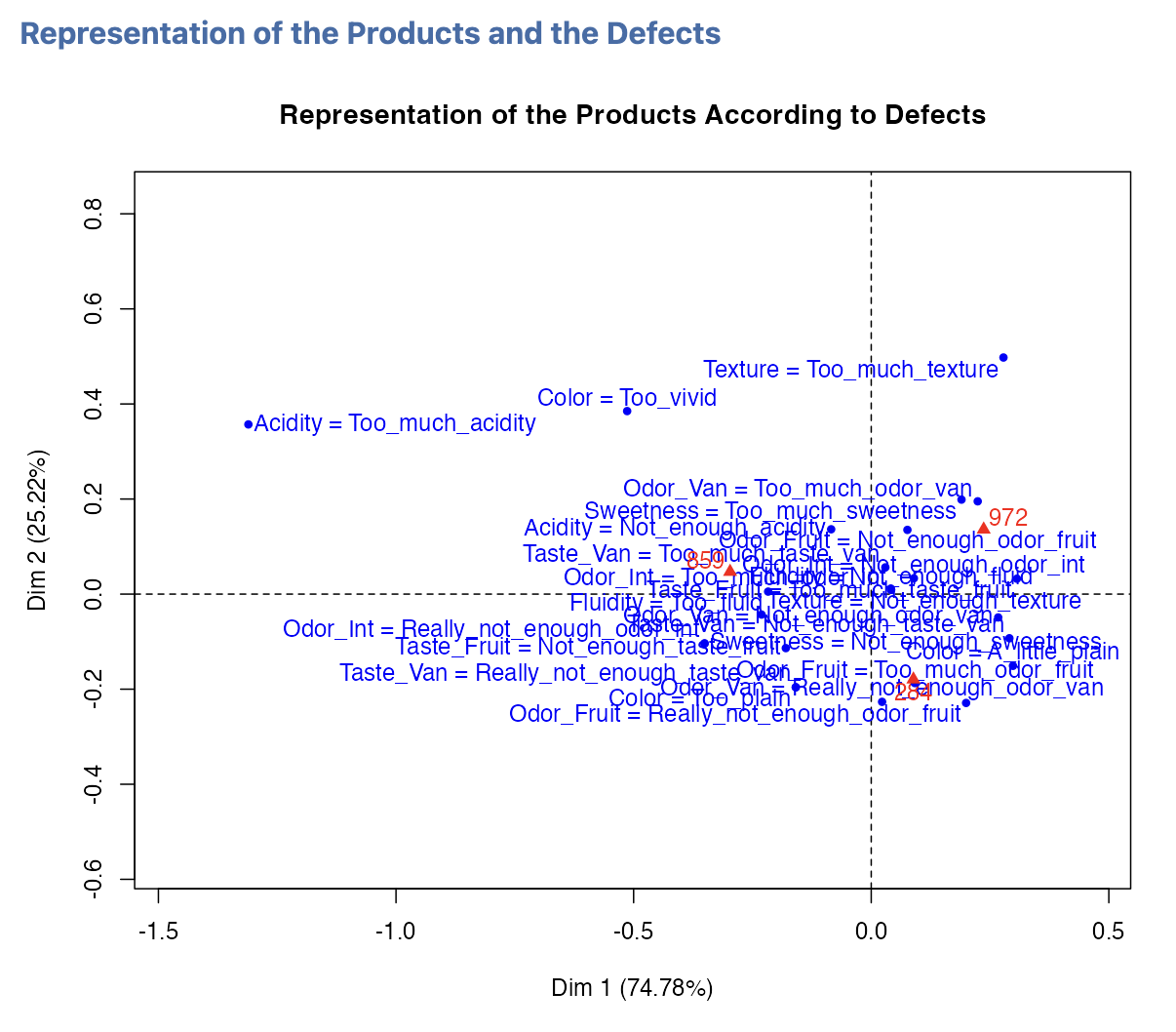
Figure 5.4: Representation of the products and the defects in the factorial plane.

The correspondence analysis is entirely summarised by the two available dimensions: Dim. 1 = 74.78% and Dim. 2 = 25.22%.

Dim. 1 mainly opposes 859 and 972, while 284 occupies a more intermediate position. The map summarises the non-JAR profile structure, but product-to-defect relationships should be interpreted relative to the factor dimensions rather than from simple row-to-column proximity.

5.7.10 Synthetic interpretation

The example mainly shows that the different pieces of JAR information are not redundant.

The global view identifies Too_much_odor_fruit as the only defect clearly associated with a liking loss across the whole product space, but this defect is too rare within each product to become a priority under the 20% threshold.

The product-specific view instead shows that extremely frequent deviations may be weakly or non-penalising: this is the case for Too_fluid and Not_enough_texture for 859. It also reveals local levers, including several deviations for 284 and especially Taste_Van — Above JAR for 972.

What we take away from this example: useful JAR analysis is not about finding “the most penalising defect”. It distinguishes what is frequent, what is globally penalising, what is specifically penalising for a product, and what combines enough frequency, effect size, and statistical evidence to become an optimisation priority.

5.8 From jamovi to the Rj Editor

Once the Rj Editor has been configured to use System R as described in Chapter 1, check R code. The generated script loads SensoMineR and FactoMineR, and uses the dataset currently open in jamovi as data.

The code successively reproduces the global multidimensional penalty with JAR(), the classical product-specific diagnostic, and the products × defects synthesis with descfreq() and CA(). It also carries over the thresholds and keyword patterns selected in the interface.

Graphics calls are written so that each product produces a separate output in the Rj Editor. No additional setting is required.

5.9 Practical tips

Always inspect JAR Coding Used for the Classical Penalty Analysis before interpreting product-specific penalties.
JAR variables must be defined as Nominal in jamovi and must contain exactly the level specified in Coding of the JAR level.
An Unclassified category indicates a Below/Above JAR grouping problem: adapt the keyword patterns before interpreting the classical analysis.
Do not confuse the two views: Global Multidimensional Penalties describes the whole product space, whereas Product-Specific Classical Penalty Analysis answers the question separately for each product.
A positive Mean drop indicates a liking loss. Interpret its magnitude together with the percentage of consumers concerned, the confidence interval, and the p-value.
Consumer threshold (%) and Mean-drop threshold are practical decision thresholds, not significance thresholds.
A frequent defect is not necessarily penalising; a strongly penalising but very rare defect is not necessarily a priority.
Use the correspondence-analysis map to understand the structure of defect profiles, not to conclude that a defect affects liking.

5.10 In summary

Use this analysis when JAR responses are available together with a liking measure and the objective is to identify deviations from the ideal level that may guide product optimisation.

SEDA first checks the JAR coding, then describes the Below/JAR/Above response frequencies, and provides two complementary views: a global penalty analysis across the whole product space and a classical product-specific penalty analysis. The multivariate correspondence-analysis synthesis completes these diagnostics by showing how products are structured according to their non-JAR categories.

Read the coding and distributions first, then the global penalties, next the product-specific penalties, and finish with the factorial synthesis.

The main point is that an optimisation priority should not rely on a single cutoff: it should combine defect frequency, mean-drop magnitude, and statistical uncertainty.